Practical Considerations of LDPC Decoder Design in Communications Systems

By Wasiela

Abstract

This paper covers some practical aspects of designing the LDPC decoder starting from comparison between different techniques, different decoders parameters or standards, the effect of those parameters on the LDPC performance, also it discusses the algorithm selection process, and floating point implementation process. The fixed point considerations in the LDPC design is covered: what is fixed-point, why we need it, how to do it, and its effect on target system design. It studies also the error floor issue of the LDPC as an example of iterative decoders, the reasons for it, how to discover the error floor and how to deal with it. A simple FPGA emulations is presented as a way to mitigate the time consuming computer simulations.

I. INTRODUCTION

The main idea of any communication system is to transmit and receive the information, between the transmitter and the receiver, respectively. When the channel, which is the environment between the transmitter and the receiver, be ideal hence the received data will be exactly the same transmitted data, and zero error in reception will be satisfied. However, in the practical environments there are impairments such as noise due to the hardware components, fading effects which may be large or small scale fading, and so on. These effects dramatically affect the communication system performance, which leads to receiving totally or partially-corrupted data. Channel coding is considered an essential component in any communication system for these purposes. The idea of channel coding is to add some redundant (parity) data and relate these data somehow with the useful information data such that we can retrieve the right useful data at the receiver. The information bits will be in length K and the codeword (information bits plus parity) will be of length N as shown in Figure 1. The ratio between K and N is defined as R=K/N < 1 which is the code-rate. When R is large i.e. closed to “1” this means we are not using stronger code. This can be chosen when the environment in the channel is not severely affecting the transmitted date hence the channel can carry a higher data-rates, and vice versa; some channel are very harmful to the signal, then we need a low coding rate (higher coding gain) to overcome the impairments of the channel.

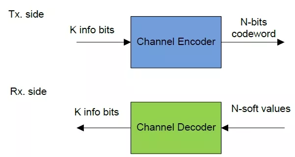
Figure 1. Channel coding idea

There are two main types of channel coding: the convolutional coding (such as Turbo codes) and the block coding (LDPC coding as an example [3]), Turbo coding is used as the main channel code for the 3G UMTS and 4G LTE cellular standards [1], [2]. LDPC code is used in WiFi, Ethernet and DVB-S2 standards [4]-[6]. Previously, due to the complexity of implementation, LDPC codes were not widely used. However, recently, LDPC coding became widely adopted in many modern standards. For example LDPC is used in 5G standard [7] due to advances of the hardware implementations, as it provides a near Shannon limit performance [3]. In our white paper we handle the design flow of LDPC coding, how to select the algorithm, and the steps to convert the algorithm starting from mathematical formulation into a real block used in the industry.

The remainder of this paper is organized as follows. Section II provides some detailed information about different LDPC codes, the floating point methodology for developing LDPC coding in the system chain and discuss the error floor phenomena. Section III provides the fixed-point design concept, the ordered steps/methodology for fixing a floating point data, then how to apply this methodology on the LDPC decoder (our case study), and finally discussing how to discover the error floor region caused by the fixed-point design in a practical manner (using FPGA prototype) instead of carrying out prohibitively long PC-based simulations.

II. LDPC DECODER

A. LDPC Tanner Graph

Tanner graphs (factor graph or a bipartite graph) are used in decoding different types of codes like LDPC codes [8]. The Tanner graph is used to represent the connection between variable nodes and parity check nodes. The variable nodes represent the symbol nodes, i.e. the received codeword that represents columns of the parity check matrix H). The parity check nodes represent the parity check equations that represent the rows of H matrix. The variable check nodes and parity check nodes are connected to each other through a set of edges. An edge links the check node i to the variable node j if the element Hij of the parity check matrix is non-null, as shown in Figure 2.

 

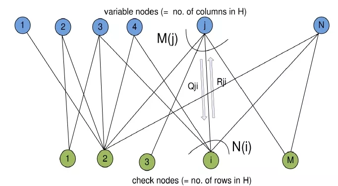
Figure 2. Tanner graph

B. Floating point design procedure and error floor of LDPC

Figure 3 shows the procedural algorithmic or floating point design of the LDPC decoder. The design steps can be divided into the following steps:

• Survey over the proposed algorithms and check the H matrix with floating point error floor: this step covers selecting the parity check matrix (H matrix) and a survey between the state-of-the-art algorithms with initial comparison with respect to the main points such as the performance, the area, the latency and the power consumption.
• Algorithm and H matrix selection: this step covers a discussion for the target performance and other comparison parameters (from the previous step) and comparing with the customer or standard requirements. (Note: H matrix selection is not valid when needed to implement a certain standard decoder, as it is mandatory to use this standard specified matrix in the decoder). The floating point error floor shall be investigated when selecting the H matrix (if applicable).
• Algorithm modeling: this step covers implementing the selected algorithm using Matlab till reaching a floating-point-working version of the model.
• Initial performance verification: this step covers initial performance verification, i.e. running some BER performance for expected target BER ~ 10-3-10-4 and compare the performance with the literature or a customer target performance with some iterations on the design if needed.
• C code implementation/update: this step covers the implemented Matlab codes to C code in order to speed up the simulations.
• Intensive performance testing: this step covers running heavy simulations for finding the performance until BER up to 10-6 - 10-8 and compare it with the target performance. Some iterations may be required if the performance at low BER did not match the target performance, hence the algorithm modeling me be revisited.
• Fixed-point design stage: this step is explained in the next section. It covers initial fixed-point design and running performance curves, then testing the error floor resulting from fixed-point design.

Error Floor of LDPC

The behavior of the BER performance of LDPC, follows a “waterfall” curves [9]. The bottom of the waterfall can experience flattened horizontal line which is referred as the error floor region in the curve, where the curve saturates at a certain performance. Error floor of LDPC can be caused at the floating point stage due to the parity check matrix construction (the code design), or at the fixed-point stage. The recommended solutions to reduce the error floor BER, at floating point stage, are by changing the construction of the parity check matrix as illustrated in [10] and [11], or by modifying the iterative decoding algorithm as proposed in [10]. For floor caused by fixed point design, careful consideration must be followed to avoid such error floor caused by the fixed point design choices.

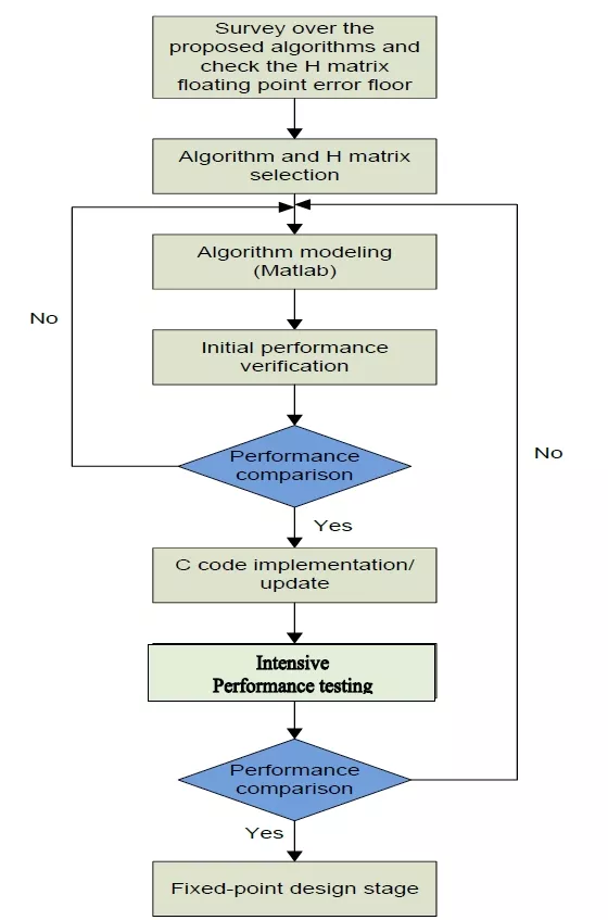
Figure 3. Floating point design procedure

III. FIXED-POINT CONSIDERATIONS OF THE LDPC

A. Introduction to fixed vs. floating point.

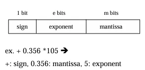
In simulation programs, program parameters are declared in single precision (32 bit) or double precision (64 bit) floating point format. In practically embedded systems H/W design like Application Specific Integrated Circuit (ASIC) the numbers shall be implemented in fixed point formats with lower number of bits in order to reduce hardware complexity and processing, on the other hand, this may lead to the effect of quantization noise. The following table (Table. 1) shows the differences between fixed and floating point representations.

Table 1. Floating point vs Fixed point representation

	Fixed point number	Floating point numbers
Representation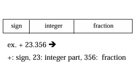
Comparison	- Lower dynamic rang + Simple hardware	+ high dynamic rang - complex hardware
Applications	Embedded systems	Graphics systems

Consequently, we need to make system simulation with fixed point for all parameters, variables or signals whether they were static or dynamic to measure the quantization noise level and how much will it affect the system performance, and select the suitable number of bits which would give acceptable performance.

Performance Measure:

As a general rule for fixed point implementation, there are two metrics to measure the performance of the fixed-point design of any block which are Signal-to-Quantization-Noise Ratio (SQNR) and Bit-Error-Rate (BER). The two performance metrics are inter-related as the SQNR affects the BER. However, for speeding-up the design process or if we have many points that need to be fixed, we may opt to do an initial fixed-point design using SQNR then test the effect on the BER performance.

The optimum way is to design the chain in order (just like the designed architecture or block diagram), however, this is not practical as each block is developed individually.

- SQNR: measures the ratio between the signal power to the quantization noise power

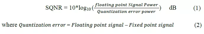
SQNR metric can be considered the dominant metric for fixed-point design of the transmitter blocks, where the BER performance cannot be applied especially if we are concerned with the design of the transmitter only. Generally, the target SQNR may be around 10-15 dB larger than the operating SNR or related to system specification, customer requirements – generally we select the value of SNR that equivalent to un-coded BER for highest constellation around 10^-3~10^-4). However, we may have an acceptable BER performance for lower SQNR values. Some iterations may be done over the design process to make sure that the design meets the requirements. If the signal is filling the full range, each bit shall contribute with ~ 6 dB in the SQNR performance.

SQNR ~ 1.761 + 6.02*n (dB), where n is the number of bits in fixed point number.

- BER:

Un-coded BER measure is used for signal chain fixed point. The BER loss for the worst case (highest constellation and worst channel) practically should not be more than 0.5 dB at the target SNR. For coded BER measure, it is used for bit chain fixed point (starting from LLR). The BER loss for the worst case (highest constellation, worst channel and highest coding rate) should not exceed 0.2~0.4 dB at the target SNR, taking into consideration that the coded target SNR differs from the un-coded target SNR.

B. Different Fixed-Point Strategies (round Vs. truncation Vs. ceiling)

There are different strategies in defining the required number of fraction bits. If we have this number "0.83388501459509”, then we have different ways to determine the required fixed-point bits for this fractional number.

Rounding:

This operation is done by round the fraction bits to the nearest number. So at this example the number

"0.83388501459509” ~ 0.833984375 (for 10 bits fraction)
"0.83388501459509” ~ 0.833892822265625 (for 15 bits fraction)
"0.83388501459509” ~ 0.84375 (for 5 bits fraction)

Truncation/Floor:

This operation is done by truncation of the fraction bits after the selected resolution. So for the current example the number shall be:

"0.83388501459509” ~ 0.8330078125 (for 10 bits fraction)
"0.83388501459509” ~ 0.8338623046875 (for 15 bits fraction)
"0.83388501459509” ~ 0.8125 (for 5 bits fraction)

Ceiling (rarely used):

This operation is done by approximate the fraction to the nearest higher number for the selected number of fraction bits. So for the current example the number shall be:

"0.83388501459509” ~ 0.833984375 (for 10 bits fraction)
"0.83388501459509” ~ 0.833892822265625 (for 15 bits fraction)
"0.83388501459509” ~ 0.84375 (for 5 bits fraction)

The rounding operation is preferred in the quantization as the quantization error due to the other operations (“ceil” and “floor”) might cause signal bias, however, it may be hardware costly. Practically, there could be a difference in SQNR between “round” operation rather than “ceil” or “floor” operation (the experiment can be done by generating random vector, then by using the three methods for quantization and calculating the SQNR for the quantized data, it is noticed that the rounded data is better than the ceiled or floored data). Ceiling operation is rarely used in fixed point design, so the most commonly used operations are rounding and truncation. Table 2 shows a comparison between the rounding and truncation operations.

Table 2. Rounding vs. truncation operations [12]

	Rounding	Truncation
PDF
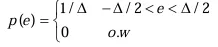
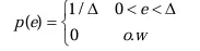
Mean square error(σ)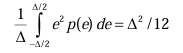
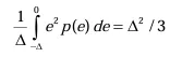	As Δ is the quantization step = 2# of bits-1.
Comparison	-Has cost of additional adder and saturator (more hardware). + has lower error.	+ Has no cost, it just truncation process. - Add bias to single (DC component). - has higher error.
How to select one of them?	If SQNR is more important than the simplicity of implementation, then rounding can be used. Only if DC bias has no effect on the original signal. i.e. if the signal on the high frequency band or it will pass through HPF (which remove DC component) and the simplicity is more important than the performance (i.e. we can recover the difference in SQNR somewhere) then the truncation can be used. For long chain of pipeline stages like FFT, you can apply truncation in the first stages and set rounder in the last or the 2 latest stages to reduce HW complexity (but the performance must be checked carefully).

C. Fixed-Point for Fraction and Integer Bits

i. Fraction Bits

The fractional number of bits should be calculated using simulation of the worst case in terms of the ranges of numbers/values (applying channel models and the different modulation techniques). As discussed above, the rounding operation shall be done for fixing the fraction bits. At each rounding operation (including input point), simulations and checking the target performance, either BER or SQNR, shall be done. Safety margin shall be considered when choosing the number of bits such that having one or two bits before the performance breaking down due to fixed point. In case of having more than one input to the block, then what is previously stated shall be applied for each input individually.

ii. Integer Bits

The main point of the Integer Bits is to avoid internal overflows of the parameters within the LDPC implementation. The internal and output integer number of bits can be calculated as the following different methodologies:

Add bits for Hardware operations:

The operations shall be handled as follows:

• Addition/subtraction: add [log2(No_Additions)] bits, to the integer part, on the largest input size, for ex. If we need to add 8 numbers each with fixed-point notation S2.5, then the resultant width will be S5.5.
• Multiplication: add the integer parts of all inputs. For complex numbers, add an extra bit for complex addition. You should also check the case of maximum negatives (rare and try to avoid) it may increase one extra bit.
• Division: add the integer part of numerator with the fractional part of denominator, however, we generally try to minimize the usage of the division operation in order to reduce complexity by using multiplication by the inverse of the denominator instead of division operation.

Guidelines for fixing a floating point variable

Givens: floating Input A (real signed)

Required: To be fixed in one sign bit + T integer bits + F fraction bits (ST.F).

Steps:

Output range shall be from (- 2^T) to (+2^T - (1 / 2F)) == [-2^T, +2^T [

1- Normalize the input to -1 to 1 (Magnitude = 1) - To simplify dealing with data - by putting binary point before all integer bits.

        A1 = A / 2^T;                           sbbb.bbbbb ➜ s.bbbbbbbb

2- Fix it in (T+F) bits; move all wanted integer and fraction bits in integer part

        A2 = A1 * (2^(T+F))                 s.bbbbbbbb ➜ sbbbbbb.bb

3- Apply rounding or truncation on undesired fraction tailing bits

        A3 = round (A2) / (2^T+F);     sbbbbbb.bb ➜ sb’b’b’b’b’b’b’.0

        A3 = floor (A2) / (2^T+F);        sbbbbbb.bb ➜ sbbbbbb.0

Rounding done by addition operation flowed by truncation, the output range may be out of input range due to carry and borrow bits resulting from addition operation which cause increasing on integer bits, i.e. x= 0.999, round(x) = 1, one more bit in integer bits. If the simulation ignore this bit it will cause growing in the # of integer bits along the program although in practical system, the H/W will truncate this additional bit and the result will be 0.0000 (causes total system failure), hint truncation doesn’t cause this problem [12]

4- Apply Saturation process

If A3 > = 1                         - overflow
  A4 = 1 – 1/ (2(T+F));             // set by maximum representable number
Elseif A3 < -1                      - underflow
 A4 = -1;                           // set by minimum representable number
Else
 A4 = A3;
End

5- Convert Normalized Fixed peak to actual Fixed peak values: A5 = A4 * 2^T;

D. Fixed-Point and error-floor.

Here we discuss the effect of the fixed-point design on the LDPC BER. Error floor of LDPC can be caused by 2 factors: the first factor is related to the parity check matrix construction (the code design), when the H matrix contains cycles or girths, this effect shall be appeared in floating point implementation, the other factor is the fixed-point design of the decoded signal which is discussed in this part. As mentioned in [4], error floor is dominated by fixed point implementation for low precision bit-widths, so it is very important to test the effect of fixation on the BER performance, it is good to mention that some standards/requirements mention Frame-Error-Rate (FER) or Packet-Error-Rate (PER) as a target performance. Actually there is no direct relation between the BER, PER and FER, however it shall be known that the target FER faces lower BER, for ex. if the target FER is ~ 10^-5, then it is expected for the BER to be in the range of 10^-7- 10^-9, which means longer simulations.

The procedure of fixing the design is shown at Figure 4, the main points in this chart can be illustrated as follows:

• Floating Point stage: this step is detailed in Figure 3, where all floating point steps are summarized and the floating point error-floor can me known.
• Fixed-Point stage: this step can be split to the following steps
  • Initial fixed-point design for the entire algorithm using Matlab and C (Matlab is preferred for the purpose of bit-level verification with the hardware, and C mainly used for running heavy simulations).
  • Obtaining initial fixed-point results for and compares them with the floating point results. Iterations on this step may be needed till satisfying the target fixed-point performance or the target loss from the floating point performance till the BER in the range ~ 10^-6 - 10^-8.
• FPGA emulation: this step covers checking the error-floor performance, actually this step shall be done after checking the floating point error floor to be sure that the only reason of the high error-floor (if found) is the fixed-point design. The block diagram of this process can be summarized as shown in Figure 5

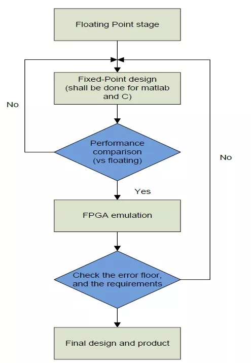
Figure 4. Fixed-point design procedure

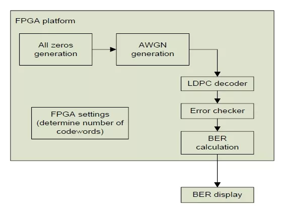
Figure 5. FPGA emulation block diagram

The target is to generate the BER performance at specifically for low BER values hence detecting the practical error floor values.

Here we use all-zeros codeword (as it is a valid codeword for block-codes) instead of implementing a random data generator and the encoder on the FPGA [13].

IV. CONCLUSION

In this white paper, we have discussed the channel coding in general with emphasis giver for the LDPC code as an example of block codes. The white paper discussed the design procedure for LDPC decoder. The main point which the white paper focused on is the fixed-point methodology, and how to apply this methodology on an actual/practical algorithm, such as the LDPC decoder and how to find the error floor limitations.

V. REFERENCES

[1] ETSI TS 125 222; Universal Mobile Telecommunications System (UMTS); Multiplexing and Channel Coding (FDD), V9.3.0 ed., 2012.

[2] ETSI TS 136 212 LTE; Evolved Universal Terrestrial Radio Access (E-UTRA); Multiplexing and Channel Coding, V13.1.0 ed., 2016.

[3] D. J. C. MacKay and R. M. Neal, “Near Shannon limit performance of low density parity check codes,” Electron. Lett., vol. 32, no. 18, pp. 457–458, aug 1996.

[4] IEEE 802.11-2012 Standard for Information Technology - Telecommunications and Information Exchange between Systems – Local and Metropolitan Area Networks - Specific Requirements - Part 11: Wireless LAN Medium Access Control (MAC) and Physical Layer (PHY), 2012.

[5] IEEE 802.3an-2006 Specific requirements Part 3: Carrier Sense Multiple Access with Collision Detection (CSMA/CD) Access Method and Physical Layer Specifications Amendment 1: Physical Layer and Management Parameters for 10 Gb/s Operation, 2006.

[6] ETSI EN 302 307-1 Digital Video Broadcasting (DVB); Second generation framing structure, channel coding and modulation systems for Broadcasting, Interactive Services, News Gathering and other broadband satellite applications; Part 1: DVB-S2, V1.4.1 ed., 2014.

[7] Samsung, “R1-162181 Channel coding for 5G new radio interface,” in 3GPP TSG RAN WG1 #84bis, Apr. 2016.

[8] Moreira, J.C. and Farrell, P.G., “Essentials of error-control coding”, Wiley Online Library, 2006.

[9] Richardson, Tom. "Error floors of LDPC codes." Proceedings of the annual Allerton conference on communication control and computing. Vol. 41. No. 3. The University; 1998, 2003.

[10] He, Yejun, Jie Yang, and Jiawei Song. "A survey of error floor of LDPC codes." 2011 6th International ICST Conference on Communications and Networking in China (CHINACOM). IEEE, 2011.

[11] Tian, Tao, et al. "Construction of irregular LDPC codes with low error floors." IEEE International Conference on Communications, 2003. ICC'03.. Vol. 5. IEEE, 2003.

[12] WASIELA team, "Float2Fixed Conversion v0.4".

[13] Zhang, Zhengya, et al. "Gen03-6: Investigation of error floors of structured low-density parity-check codes by hardware emulation." IEEE Globecom 2006. IEEE, 2006.