Shrinking LLMs with Self-Compression

By Jakub Przybyl

July 3, 2025

Language models are becoming ever larger, making on-device inference slow and energy-intensive.  A direct and surprisingly effective remedy is to prune complete channels whose contribution to the task is negligible.  Our earlier work introduced a training-time procedure – Self-Compression [1, 4] – that lets back-propagation decide the bit-width of every channel, so unhelpful ones fade away. This simultaneously reduces parameters, numerical precision, and even the number of tuneable hyper-parameters, yet leaves predictive quality intact.

When we extended the same idea to a transformer [5], we noticed something intriguing: when a channel’s learned precision slips all the way to zero bits, the resulting model becomes even more compact than one restricted to a fixed ternary code.  Because the method touches only standard linear layers, the compressed network can deliver performance gains on CPUs, GPUs, DSPs, and NPUs without modification to the runtime stack, offering a single lightweight model for general deployment.

In this work, we take the idea further still with a block-based sparsity pattern. The sections that follow describe how Self-Compression is woven into the baseline model, examine the weight patterns it produces, and discuss implications for resource-constrained deployment.

Self-Compressing an LLM

Our reference model is nanoGPT [2], a compact GPT variant trained on the shakespeare_char corpus. With about 11 million trainable parameters, the model is small enough to run quickly, yet large enough to expose the full transformer computation pattern.

The model contains:

• An embedding of each token to a multidimensional vector.
• Six identical transformer blocks with causal multi-head attention (including input and output linear layers), layer normalisation, and a feed-forward module containing a further two linear layers.
• An output stack comprising a final layer normalisation, a linear layer, and a softmax outputting probability over the possible output tokens.

In transformer networks, over 90% of the weights – and therefore the bulk of memory bandwidth, DRAM consumption and power usage – reside in the four large linear layers within the transformer blocks. For our experiments, we therefore only targeted self-compression at those layers, leaving the remainder of the baseline model unchanged.

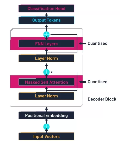
Quantised transformer architecture, based on a figure from [3], modified by author.

Later sections analyse the sparsity that emerges across blocks and channels. Understanding which layers go sparse first provides useful insight into which layers of an LLM may be less important. This may allow targeting of future optimisations where redundancy naturally accumulates.

How Self-Compression Works

Self-compression [1, 4] lets the network learn its own width and precision as part of conventional neural network training. Every output channel is quantised by a differentiable function.

where bit depth b≥0  and scale exponent e are learnable parameters in the same sense as neural network weights.  A straight-through estimator treats the rounding derivative as 1, so that b and e receive normal gradients. This is easy to implement in a DL framework like PyTorch.

Training minimises the original task loss L₀ , but we include an extra size penalty Q .

where Q is the average bits stored in the model, and  is a penalty term chosen by the user.

For appropriate choice of y, the method retains baseline accuracy while cutting total model bits, all within an otherwise standard training setup.

Weights after Self-Compression

As training progresses, we see the number of bits remaining in the network decreasing along with the validation loss. After starting training by assigning 4 bits per weight, it reduces by half within a few hundred epochs, going on to settle over time at around 0.55 bits per weight.

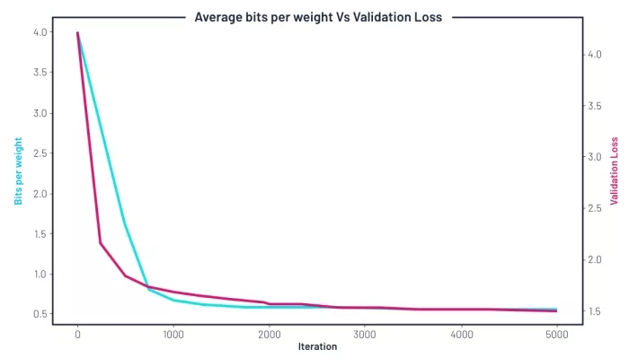
Change of average bit-width (blue, left axis) and validation loss (red, right axis) during training with a compression penalty .

Things get more interesting still when we look at the sparsity rate, and how it changes with depth. Sparsity increases as we go deeper into the model. This suggests that later layers are less information dense. We observe the linear layers in the attention module become the sparsest in deeper blocks, with more than 95% of weights in blocks 4 and 5. The feed-forward layers also become very sparse, with about 85% of weights removed. By contrast, the first block (0) keeps over half of its weights, likely because early layers are important for capturing basic patterns in the data.

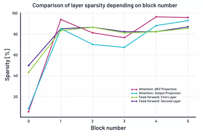
Sparsity (percentage of zeroed-out weights) of each linear layer in all transformer blocks.

If this generalises to other language models and tasks, then it’s possible that a performance saving can be obtained even without self-compression, simply by reducing the number of features towards the end of the network.

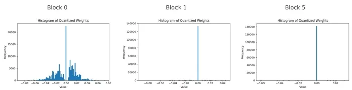
Histograms of quantised weights for the first feed-forward linear layer in blocks 0, 1, and 5.

When we look at the histograms of weights across all three blocks, we see the non-zero weights are grouped around small values close to zero, especially in the deeper blocks. This shows that even when a weight is not zero, the model prefers to keep it small. The deeper the block, the fewer large weights remain. This shows that the model avoids making up for the loss of channels by increasing the size of the remaining weights.

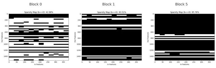
Binary masks showing pruned (black) and kept (white) weights in the first feed-forward linear layer of blocks 0, 1, and 5.

The sparsity masks show how the pruned weights are arranged. In block 0, the pruning is spread out, with small gaps and thin lines showing individual channels removed. In block 1, larger groups of weights are pruned together, forming horizontal bands where whole output channels are gone. By block 5, most of the layer is pruned, with only a few channels left.

Conclusion

Self-Compression [1, 4] reduces both the bit-width and the number of active weights, while creating patterns like channel sparsity that are easy to understand and efficient to use on hardware. Early layers stay mostly dense to keep important information, while deeper layers become highly sparse. The few remaining weights stay small and close to zero. These results show that Self-Compression helps build models that are smaller, faster, and ready for use in resource-limited settings like edge devices.

The experiments presented here confirm that Self-Compression can successfully shrink a transformer model, in this case a nanoGPT [3] trained on character-level Shakespeare dataset, without harming its predictive quality. By letting the model decide which channels and weights to keep, the method avoids unnecessary manual tuning and produces a clean block-sparse structure that is easy to deploy on CPUs, GPUs, NPUs, and other hardware. This means that the same compact model can serve across the entire edge stack without further modifications.

Future work could explore applying this method to larger language models, multi-modal transformers, or models fine-tuned for specific tasks, as well as combining Self-Compression with other techniques like knowledge distillation to push efficiency even further.

References

[1] Szabolcs Cséfalvay and James Imber. Self-compressing neural networks.
arXiv preprint arXiv:2301.13142, 2023. URL https://arxiv.org/abs/2301.13142.

[2] Andrej Karpathy. Nanogpt.
https://github.com/karpathy/nanoGPT, 2023.

[3] Sahitya Arya. Mastering decoder-only transformer: A comprehensive guide.
https://www.analyticsvidhya.com/blog/2024/04/mastering-decoder-only-transformer-a-comprehensive-guide/, 2024

[4] Szabolcs Csefalvay. Self-compressing neural networks.
https://blog.imaginationtech.com/self-compressing-neural-networks, 2022.

[5] Self-Compression of Language Models for Edge Inference, Edge AI Milan 2025
https://site.pheedloop.com/event/milan2025/sessions/SESYFUFEHW3Q3B0RE