Your FPGA prototype runs. Can you see inside it?

By Exostiv Labs

October 19, 2026

An FPGA prototype runs faster than an emulator and produces far more data than any debug tool can hold. Add several chips and several clock domains, and seeing the whole system — on any board — becomes the real problem.

Speed and realism are the reasons why we build FPGA prototypes. An emulator runs at its own maximum frequency, whatever the design. A prototype on AMD Versal or UltraScale+ can run at several hundred MHz, close to target speed, with real software, real interfaces and real peripheral traffic over long runs. That same speed is where visibility starts to break down.

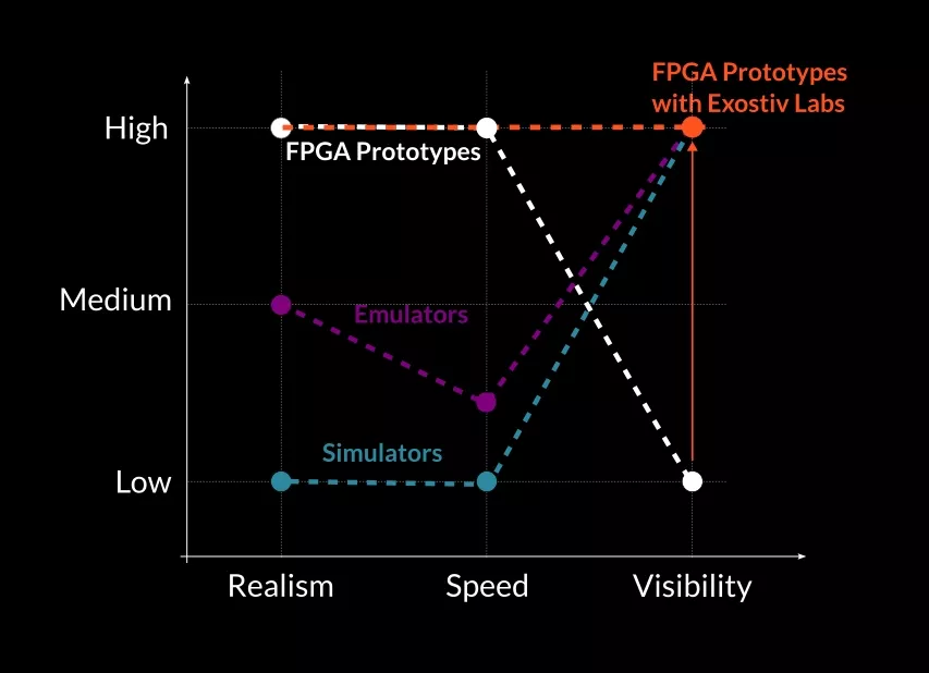
At several hundred MHz, the design generates a gigantic amount of internal signal data. Something has to capture it, store it and make it readable, and that is already a fundamental engineering challenge. Spread the design over several FPGAs and clock domains and it gets worse: there is more data than any single capture window can hold, and each source runs on its own time base. Having to build an understanding from scattered data sources of the same whole assembled system will slow you down. Conversely, seeing the whole system intuitively — naturally can we say — is what allows you to be productive during FPGA prototyping.

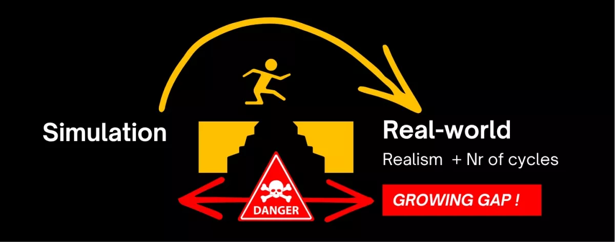
So the visibility gap widens as designs grow. The bugs that cost the most time usually sit right in it.

Where the gap comes from

The first limit is capture depth. JTAG-based tools store samples in on-chip BRAM, which the design also needs. The observation window typically ends up in the microsecond range. Many prototype failures need far longer to show up: timing issues that accumulate over thousands of cycles, synchronization drift that grows frame after frame, interface behaviour that only appears under real load. A window of a few microseconds won’t catch them.

The second limit is frequency. Designs don’t all run at the same speed. A large SoC split across many FPGAs runs slower because of inter-FPGA timing constraints. A complex design on one to four FPGAs, with little partitioning, can reach several hundred MHz. The debug infrastructure must follow the design across that whole range. It should never be the thing that sets the ceiling.

The third limit is system fragmentation. With several clock domains and several FPGAs, each capture source records data on its own time reference. Look at the domains one at a time and cross-domain behaviour disappears: the timing between interfaces, the interactions between subsystems. Until now, getting a single coherent view meant hand-written scripts, detailed knowledge of how the instrumentation was set up, and the same effort again for every capture session.

Turning transceivers into debug highways

Exostiv sends captured signals out through the FPGA’s own high-speed transceivers to external storage. The BRAM limit goes away. Captures hold gigabytes of signal history, organized in large chunks that can be stopped and restarted, so the total observation span follows real operating conditions instead of tool limits. Capture runs at the design’s actual operating frequency, from slow partitioned multi-FPGA systems up to several hundred MHz on AMD Versal or UltraScale+.

A small debug IP, inserted through the standard Vivado flow, handles the instrumentation with little FPGA resource overhead. Since the link goes through transceivers rather than proprietary hardware, Exostiv works on any board that carries an AMD FPGA: AMD evaluation boards, third-party prototyping platforms or fully custom hardware.

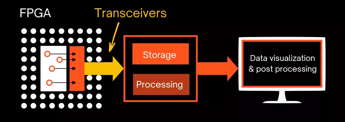
Since the link goes through transceivers rather than proprietary hardware, Exostiv works on any board that carries an AMD FPGA — AMD evaluation boards, third-party prototyping platforms or fully custom hardware. No dedicated platform required.

Maestro: one view of the whole system

Deeper capture doesn’t fix fragmentation. That takes a layer that hides the instrumentation itself.

Maestro, part of Exostiv Software, does that job. It collects project data from every Exostiv IP instance in the design, whatever the number of clock domains or FPGAs. It runs a master/slave trigger scheme across all capture sources. Then it merges every data set into one synchronized waveform view on a common timescale.

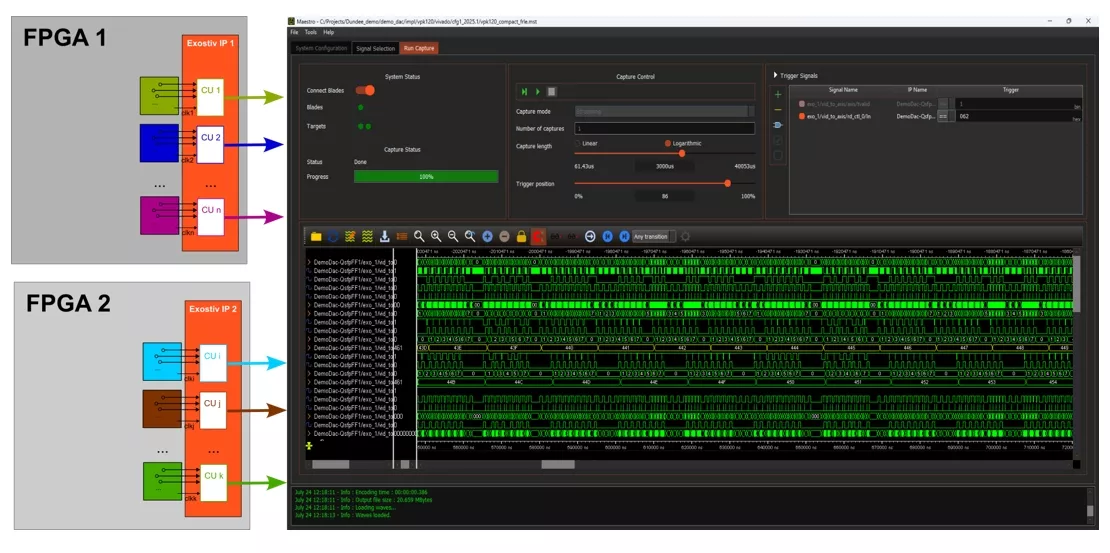The engineer sees the system as a whole, with every clock domain, subsystem and interface on the same timeline. Whoever analyzes the capture doesn’t need to know how the IP was inserted, or by whom. The capture layer fades into the background. What’s left is the system, running under real conditions, observable across every domain and every cycle that matters.

A case: a fault that takes 90 seconds to build

Take an SMPTE ST 2110 IP video gateway on AMD UltraScale+, carrying more than 40 Gbps of live streams. The symptom is lip sync drift: audio and video slowly separate during long runs. Simulation is clean. The fault needs 1,000 to 5,500 frames to become visible, which means 17 to 92 seconds at 60 fps, depending on conditions.

The JTAG capture window was 110 µs. The observation time needed was over 90 seconds, roughly 840,000 times what a JTAG-based tool could provide.

The team ran Exostiv in pre-trigger mode, the dashcam approach. More than 400 bits of sync logic, timestamps and state were recorded from the 148.5 MHz clock domain, with storage qualification keeping about 27,500 samples per frame. When the drift showed up on the monitor, the operator stopped the capture. The 8 GB circular buffer froze on the spot, with the previous 5,500 frames already inside. The whole run-up to the fault was there.

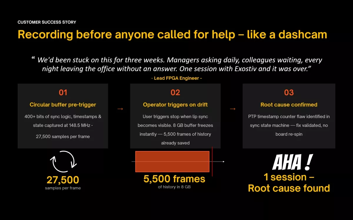
The root cause was a flaw in the PTP timestamp counter of the sync state machine. The team validated the fix in the same session. No board re-spin.

“We’d been stuck on this for three weeks. Managers asking daily, colleagues waiting, every night leaving the office without an answer. One session with Exostiv and it was over.”
— Lead FPGA Engineer

What changes

The gap between simulation and a real prototype is not new. Its size is. More clock domains, more FPGAs and more data mean standard tools see a shrinking share of what needs validating. Exostiv covers that gap end to end: deep capture where BRAM-based tools stop, full operating frequency across the speed range, a single system-level view with Maestro across chips and clock domains, and board-agnostic deployment — on any AMD FPGA board, without a dedicated platform.

Exostiv Labs is an AMD Embedded Silver Partner. Exostiv Probe and Exostiv Blade support any AMD FPGA device with high-speed transceivers, through the standard Vivado flow.

Request a demo at exostivlabs.com.