ChiPy®: Bridge Neural Networks and C++ on Silicon — Full Inference Pipelines with Zero CPU Round-Trips

The ChiPy DSL is Quadric's Python framework for building complete on-chip pipelines. Using YOLOX-M as a case study, we show how backbone inference, box decoding, and NMS run entirely on the Chimera GPNPU — no host CPU intervention, no DDR round-trips, just Python compiled to silicon.

The Split Pipeline Problem

Every object detection deployment hits the same wall. The neural network backbone runs on an accelerator — GPU, NPU, DSP — and then the results get shipped back to a host CPU for postprocessing. Box decoding. Score filtering. Non-Maximum Suppression. The stuff that turns raw tensor output into actual detections.

This round-trip is not a minor inconvenience. NMS alone can consume 30-50% of total pipeline latency in edge deployments. The data has to leave the accelerator's local memory, traverse a bus to main DDR, get picked up by the CPU, processed through branching scalar code that NPUs can't touch, and then the final results travel back. Every frame. Every inference.

The root cause is architectural: traditional NPUs handle matrix multiplies and nothing else. The moment your algorithm needs a comparison, a branch, a sort, or a loop with a dynamic termination condition, you're back on the CPU. Detection pipelines need all of these.

The Chimera GPNPU handles MAC operations, vector math, scalar control flow, and branching logic in a single unified core. That architectural difference is what makes the rest of this post possible.

Enter the ChiPy DSL

The ChiPy DSL is Quadric's Python framework for tensor-level computation on the GPNPU. If you've used JAX, the mental model maps directly: the ChiPy library operates at the tensor level with NumPy-like syntax, while the lower-level Chimera Compute Library (CCL) handles kernel implementation, analogous to how Pallas sits beneath JAX.

The key properties:

• NumPy-like syntax with operator overloading. Write array operations the way you already do.
• Dual execution. The same ChiPy DSL code runs on your CPU for validation and compiles to GPNPU for deployment. Zero code changes between test and production.
• ONNX integration. Import quantized models directly. The Chimera Graph Compiler (CGC) handles backbone compilation; the ChiPy tool wires it together with your custom pre- and post-processing.
• Two decorators, full pipeline. @chipy.ccl_custom_op bridges a C++ CCL kernel into the Python graph. @chipy.func defines the top-level pipeline that chains everything together.

That last point is the critical one. The ChiPy compiler doesn't just run neural networks. It composes entire application pipelines — preprocessing, neural inference, postprocessing — into a single compiled program that executes on-chip without returning to the host.

Here's what the decorator pattern looks like:

@chipy.ccl_custom_op(
    kernel_source="yolox_postprocess.hpp",
    kernel_name="yolox_postprocess",
)
def yolox_decode_nms(cls_scores, bbox_preds, obj_scores):
    # Python body: CPU reference implementation
    # Runs identically on CPU for testing
    boxes, scores, classes = decode_proposals(cls_scores, bbox_preds, obj_scores)
    keep = nms(boxes, scores, iou_threshold=0.45)
    return boxes[keep], scores[keep], classes[keep]

The @chipy.ccl_custom_op decorator does two things at once. During CPU testing, the Python body executes directly — you can validate against reference outputs with standard tooling. When compiled for the GPNPU, it swaps in the optimized C++ kernel specified by kernel_source. Same interface, same results, different execution target.

YOLOX-M End-to-End: The Full Pipeline on Silicon

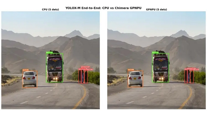
To make this concrete, here's a complete YOLOX-M detection pipeline running entirely on the Chimera GPNPU. No host CPU involvement after the input image is loaded.

Model specs:

Parameter	Value
Model	YOLOX-M (25.3M params)
Input	640 x 640, int8 quantized
Dataset	COCO 80-class
Pipeline	Backbone (CGC) + Decode + NMS (CCL)
Target	Chimera GPNPU (8 cores, 16 MACs/PE, 8 MB OCM)
Quantization	Asymmetric int8 activations, int8 weights

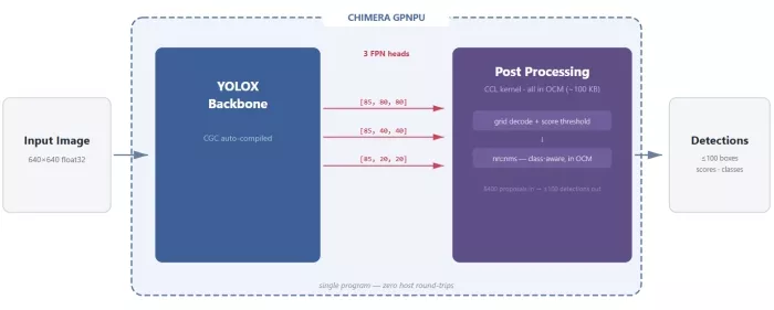
The pipeline has two stages. The backbone (compiled by CGC from a quantized ONNX model) produces three Feature Pyramid Network heads with classification scores, bounding box regressions, and objectness scores. The CCL custom op then decodes all 8,400 proposals, applies score filtering, and runs NMS — all in a single kernel invocation.

Here's how the ChiPy DSL wires it together:

@chipy.func
def yolox_e2e(input_image):
    # Stage 1: Backbone inference (CGC-compiled ONNX model)
    cls_out, bbox_out, obj_out = yolox_backbone(input_image)

    # Stage 2: Decode + NMS (CCL custom op)
    boxes, scores, classes = yolox_decode_nms(cls_out, bbox_out, obj_out)

    return boxes, scores, classes

Five lines. The yolox_backbone call is a CGC-compiled graph. The yolox_decode_nms call is the CCL custom op defined above. ChiPy compiles both into a single GPNPU program. Data flows from backbone output directly to the postprocessing kernel through on-chip memory. No DDR round-trip. No host CPU context switch.

Under the Hood: Why This is Fast

The CCL kernel that handles decode and NMS is where the GPNPU architecture pays off. Here's what happens inside yolox_postprocess.hpp:

Decode

Each of the three FPN heads (stride 8, 16, 32) produces proposals at grid positions. The kernel decodes bounding box coordinates from grid offsets and applies the exponential width/height transform, operating on all proposals for a given head before moving to the next. The GPNPU's scalar ALU handles the coordinate math natively — no need to ship this to a CPU.

Score Filtering

Objectness scores multiply class scores to produce final confidences. Proposals below the confidence threshold are discarded immediately. This is branching, data-dependent control flow — exactly the kind of work that stalls a traditional NPU pipeline.

NMS

The surviving proposals are sorted by score. The kernel iterates through them, computing IoU (intersection over union) between each candidate and all previously accepted detections. Boxes with IoU above the threshold are suppressed. This is a nested loop with dynamic termination — textbook CPU work that the GPNPU executes at full speed because its processing elements include scalar units alongside the MAC array.

All 8,400 decoded proposals fit in the GPNPU's on-chip memory. The entire decode-filter-NMS sequence executes without a single DDR stall. Each FPN head is processed and its memory freed before the next head loads, keeping the OCM footprint minimal.

Why This Matters

Three things make this significant beyond a single demo.

Deterministic Latency

The GPNPU uses software-managed scratchpad memory, not hardware caches. No cache misses, no variability between frames. The execution time for the postprocessing kernel is the same on frame one and frame ten thousand. For safety-critical deployments — ADAS, industrial inspection, robotics — this predictability is a requirement, not a feature.

The Pattern Generalizes

ChiPy's composition model works for any detection architecture. The 26.02 SDK ships with both YOLOX-M and RetinaNet end-to-end demos using the same @chipy.ccl_custom_op + @chipy.func pattern. The RetinaNet pipeline goes further, adding preprocessing (crop, resize, normalize) as additional CCL custom ops, all composed in a single compiled program. Any model that follows the backbone-plus-postprocessing pattern can be wired up the same way.

No C++ Required for Pipeline Work

The CCL kernels are C++ (and will remain so for performance-critical inner loops), but the pipeline composition layer is pure Python. Engineers who can write NumPy can build full on-chip detection systems. The @chipy.func decorator abstracts the compilation, memory management, and data routing between stages.

---

Explore NPU IP:

• GPNPU Processor IP - 32 to 864TOPs
• Safety Enhanced GPNPU Processor IP
• GPNPU Processor IP - 4 to 28 TOPs
• GPNPU Processor IP - 1 to 7 TOPs

---

---

This is what "general-purpose" means in practice. Not just matrix multiplies. Not just neural networks. Full application pipelines — the kind that actually ship in products — running on a single processor with a single programming model.

Explore the complete YOLOX-M and RetinaNet end-to-end tutorials in Quadric Dev Studio.